Monitoring the Mattermost server with Prometheus and Grafana

Lately we’ve been working on improving different parts of the Mattermost server, including our monitoring and observability capabilities.

We’ve been using Prometheus and Grafana to monitor our cluster for a while now, and you can read this great post where my colleague Stylianos explains how we have them working for our multi-cluster environment. 

In this post, I’m going to talk about how we work with metrics and observability from the server-side of Mattermost and what we did recently to improve it.

We need to understand the health of our application so we can benefit from some practices coming from the SRE world that would help us achieve that objective: the four golden signals and the RED method.

What are the four golden signals?

The four golden signals come from the SRE book that was written by the Google SRE team and served as the first introduction to the SRE concept.

Basically, it says that if you can only measure four metrics on your systems, you should focus on these four:

1. Latency

How long does it take for your service to process a request? To determine latency, we have to distinguish between successful and failed requests and track both of them.

2. Traffic

How much traffic is our service receiving? Traffic should be measured using an adequate metric that makes sense for the kind of service we have. For example, if your system is a web service, the metric should be requests-per-second. In other cases (e.g., ecommerce), the metric could be the number of transactions.

3. Errors

How many errors are your systems facing and how many of them are different? For example, we might have 500 errors, and 200 of them come from serving the wrong content or even by some kind of business rule, like serving requests below a predefined threshold.

4. Saturation

How full is your service? This is a tricky one because you have to find and define a metric that alerts you when your service’s capacity is exceeded.

To do this, you have to figure out which resources of your service are more constrained (e.g., memory or CPU) and monitor those. You also need to be aware that sometimes a service starts degrading before it reaches 100% utilization.

Bottom line: If you receive alerts based on these four rules, your system would be decently monitored. (You can always monitor additional metrics, too.)

But do we have a more simple and explicit way to implement these rules for a request-driven service? Yes, and it’s called the RED method.

What is the RED method?

The RED method, which was originally designed for microservices, is an acronym that outlines three key metrics every service should measure.

1. Rate

The rate refers to the number of requests per second your service is handling.

2. Errors

Errors are the number of failed requests per second. This includes all of the types of erroneous requests.

3. Duration

Duration refers to how long it takes to serve a request and its different distributions (e.g., p50 and p99).

As you can see, these are more straightforward rules meant to be used for monitoring request-driven services. They are based on the four golden signals but have been simplified to make it easy to implement for all the services you have.

There is another method based on the acronym USE. But it’s more focused on monitored resources. The USE method, however, was part of the spark that led to creating the RED method.

As a final note, saturation is excluded from the RED method because it is a more advanced case. Still, it is useful, and once we have a clear picture of our system, we’ll include it.

What is Prometheus?

Now that we have a better understanding of the foundation that is going to guide our monitorization system, we need to start working with the metrics.

In Mattermost Enterprise Edition, we collect metrics from our server and send them to Prometheus. Prometheus is a systems monitoring and alerting toolkit built in Go, which makes it very easy to install and/or upgrade.

Prometheus has a wide range of service discovery options, as you can see here, allowing you to discover your services and start collecting metrics from them.

But how does Prometheus get the data? Even though Prometheus is able to receive pushed metrics,  it’s better to work on a pull basis. That means that your service should expose an endpoint where Prometheus calls to retrieve the associated metrics regularly.

It’s important to know what Prometheus is capable of. At the same time, it’s just as important as to know what the service doesn’t do:

• Prometheus doesn’t provide logging capabilities, which are as important as the monitoring itself. In our case, we’re using ELK for logging.
• Prometheus doesn’t provide long-term storage capability in its local storage, which is not clustered or replicated. But you can use their remote storage integrations to overcome this limitation. Another possibility is using Thanos.
• You don’t get automatic horizontal scaling, but there are ways to scale Prometheus. Here are some examples. 

Prometheus stores the data in its internal time series database with its format. But at the client/library level, the service provides four basic types of data—counters, gauges, histograms, and summaries—which we’ll examine next:

• Counters are cumulative and are a single monotonically increasing counter meaning that must be used to reflect metrics that are always increasing—like requests and errors. If you need to handle values that can decrease, you should use gauges.
• Gauges store values that can increase or decrease. For example, it can be used to reflect connections or memory usage.
• Histograms are usually used to display information visually, like request durations or sizes, for example. A histogram is composed of three parts:
  • The total sum of all the values
  • The number of events that have been observed
  • Cumulative counters stored as buckets
• Summaries are similar to histograms, but the main difference is that this type stores configurable quantiles instead of buckets.

For better or worse, one of the most well-known characteristics is the query language PromQL. Despite it being a very powerful tool, it’s also a bit hard to understand at times. To illustrate:

sum(increase(api_time_count{server=~”server_name”,status_code!~”(2..|3..)”}[5m])) by (status_code, instance)

One thing that is worth mentioning is that Prometheus creates a multidimensional metrics system using labels. As you can see in the previous example, you can have the same metric but for different servers and status_codes using only the metrics that you send. This is one of the most powerful features of Prometheus.

Using those labels, we’re able to aggregate and group by metrics. In the example query, we’re using the sum function which aggregates the results grouped by the provided label names, in this case status_code and instance in that order.

Once you are familiar with Prometheus, you can perform very interesting and useful queries, as you will see in the next section.

How does Mattermost use Prometheus?

Now that we know what Prometheus is and how it works, it’s time to explore the metrics we have at Mattermost.

One of the good things about this method is that it requires just one metric which is very easy to obtain. In our case, we have a histogram called api_time that stores the time it takes to serve an API request.

At this point, we should talk a bit about histograms on Prometheus. The first thing you should know is that they should be used sparingly—as recommended by Brian Brazil in his fantastic talk about how counters work. But why? Histograms are stored in buckets and those buckets are expensive. 

Another recommendation about histograms is to use up to 10 buckets and define them and their width. So, at first, you’re probably going to start using the default buckets, as we’re doing. But that leads to a possible future problem: corruption of the histogram data. 

Once you have a clear picture of what your system boundaries are, you need to change the default buckets and start using your own to adjust them better to your system. At that point, we’re going to face corruption in our histogram data when we select a time range wide enough to mix the old data with the new. You can read a bit more about the problems with histograms in this post.

Before we talk about the dashboard and the queries, I want to make a brief comment on two counter functions: increase and rate.

Prometheus has different data types: instant vector, range vector, scalar, and string. In our case, we’re going to center on the instant and range vector. If you want to show data in a graphic, you need an instant vector. But, usually, you want to show the rate of some metric (e.g., the per-second rate of HTTP requests) and that is when rate or increase enters in the equation.

The rate function takes a range vector and returns the per-second average rate of the time series in the range vector. On the other hand, the increase function is syntactic sugar for the rate function but multiplied by the number of seconds in the time range provided. 

So, if you need to show the per-second rate for a metric, you should use rate or irate in case you are graphing fast-moving counters. But if you don’t need a strict per-second graphic, the documentation recommends you to use increase because it’s easier to read.

How does Mattermost use Grafana?

We’re building our dashboards using Grafana. It provides a connector, i.e., a “data source” as it’s called in Grafana, which makes it very easy to create graphics and dashboards using our stored data.

There are two important things to know about the use of Grafana with Prometheus: scrape interval and step.

In the Prometheus data source configuration, you should set the scrape interval because that configuration affects one important parameter: Min time interval. And this parameter sets the lower limit to both the $__interval variable and the step parameter of Prometheus range queries.

And what is the step parameter? It’s a Prometheus parameter that defines the query resolution step width. We should be careful with this parameter because if we set the rate below the step parameter, we’re going to discard half of the data. So, the recommendation is to make sure your rate range is at least your step for graphs.

Grafana provides also two special variables: $__interval and $__range :

• $__interval variable is roughly calculated as the time range (to-from) divided by the step’s size. This variable provides you with the ability to plot dynamic graphs. There is also the milliseconds version: $__interval_ms.
• $__range represents the range in the current dashboard and is calculated as to – from. It also has the milliseconds version. We’re using this variable to get values for all the time ranges, for example.

One common question is this: What range do I have to use in my range queries? Well, there is no silver bullet for that. Usually, the recommendation is to set a range at least two times the scrape interval. But the result depends on the data you’re receiving, so you have two options:

• Create a variable with different range options
• Use the $__interval variable

Pick the one that fits better with the data you’re receiving at that time.

Queries and panels

And finally, the easy part: creating the panels and the queries!

To create the dashboard, we need three panels: Rate, Errors, and Duration.

Rate

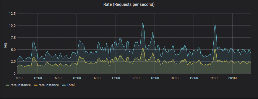
sum(rate(api_time_count{server=~”$server”}[5m])) by (instance)

The Rate query gets the rate, per second, which is why we’re using the rate function of the queries we’re receiving, grouped by server instance at five-minute intervals.

We’re also using the sum function which aggregates the results grouping by the provided label name, in this case instance.

Errors

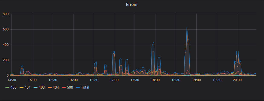
sum(increase(api_time_count{serverallation=~”$server”,status_code!~”(2..|3..)”}[5m])) by (status_code, instance)

For the Errors query, we don’t need to get the data on a per-second basis. So we use the increase function to get the number of requests that returned error responses.

Duration

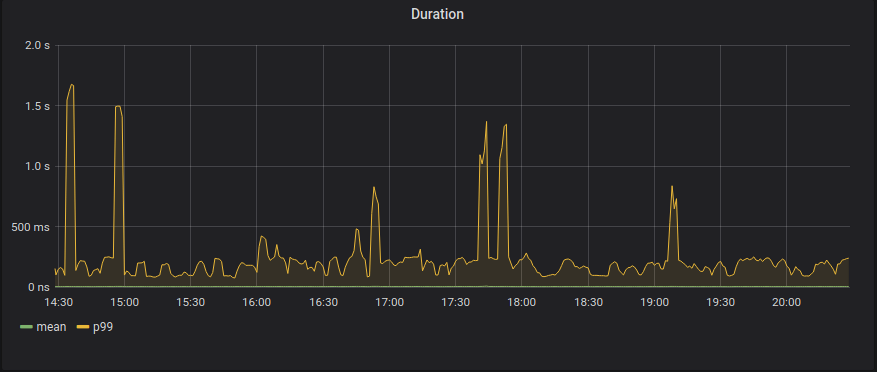
histogram_quantile (0.50,sum by (le, instance(rate(api_time_bucket{server=~”$server”}[5m])))

histogram_quantile (0.99,sum by (le, instance(rate(api_time_bucket{server=~”$server”}[5m])))

Finally, for the Duration panel, we’re using the histogram_quantile function to calculate the mean, 50th percentile, and the 99th percentile grouped by instance.

There is a special term, le. It means less or equal and that is because, as we’ve said before, the histograms in Prometheus are cumulative.

But this is just the beginning. There are plenty of things you can include in your dashboard. For example, you can add alerts using Grafana that checks for your SLO or even you can approximate the Apdex score.

Conclusion

This is a brief introduction to what we’ve done to improve the monitoring of our server service. It’s worth mentioning that we’re still learning about the Prometheus/Grafana world, so if you read something wrong or misleading, please contact me.

Last but not least, I want to thank all the help I’m receiving (Justin Reynolds, Claudio Costa, Eli Yukelzon, Javier Gamarra, Alex Guirao, and Rafa Casado) in reviewing and correcting this post :).